
Conditional formatting is a attribute in Google Sheets during which a cell is formatted in a selected process when apparent circumstances are met. The formatting can embody highlighting, bolding, italicizing – superior about any seen changes to the cell.
Simply because it is also carried out for the cell you’re at present in, conditional formatting may maybe maybe be disclose based totally solely completely on circumstances met in a single different cell.
![→ Get cling of entry to Now: Google Sheets Templates [Free Kit]](https://no-cache.hubspot.com/cta/default/53/e7cd3f82-cab9-4017-b019-ee3fc550e0b5.png)
Let’s dive into simple the machine to fabricate this situation based totally solely completely on a pair of requirements.
How Conditional Formatting Works
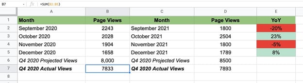
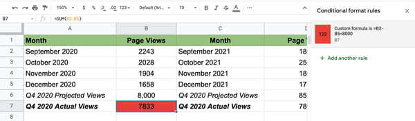
To be taught tips on learn how to disclose conditional formatting, let’s disclose this workbook for example.
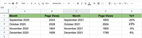
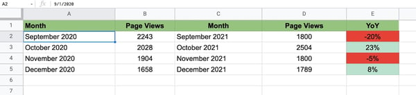
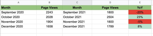
It’s a workbook displaying internet clarify visitors twelve months over twelve months from This fall 2020 to This fall 2021, with the web page views together with the twelve months-over-twelve months share substitute.
Right here’s what we’re searching to hold out right here: When the proportion substitute is simple YoY, the cell turns inexperienced. When it’s detrimental, the cell turns pink. This makes it simple to acquire a mercurial effectivity overview earlier than diving into the precept factors.
Listed below are the steps to disclose the conditional formatting.
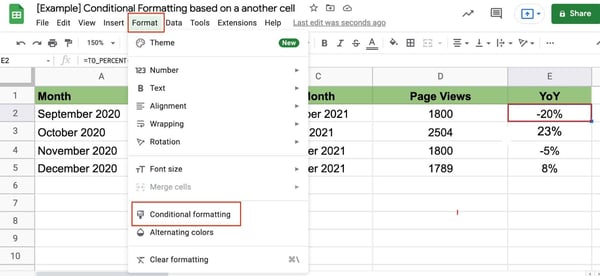
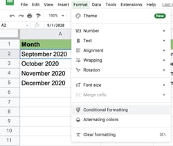
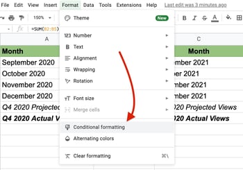
1. Seize the cell that you just may properly very successfully be searching to format, click on on on “Construction” from the navigation bar, then click on on on “Conditional Formatting.”
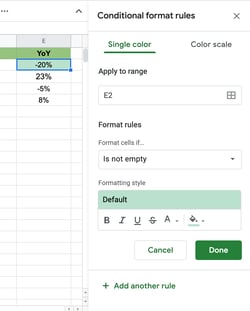
2. Whereas staying inside the “Single color” tab, double-take a have a look at that the cell under “Follow to vary” is the cell that you just may properly very successfully be searching to format. 
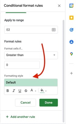
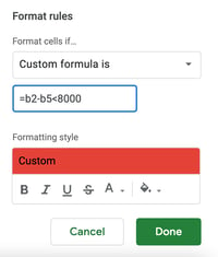
3. Plot your format concepts.
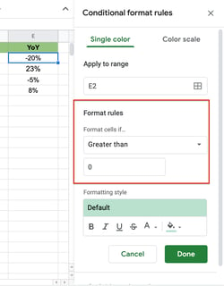
It is going to robotically default to a worn conditional formatting system. On this case, originate the dropdown menu under “Construction cells if…” to to seek out your concepts. Alternate options will ogle as follows:
4. Use your formatting mannequin, then click on on “Accomplished.”
5. Verify the rule modified into as soon as utilized under “Conditional Formatting Tips.”
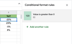
6. Add one different rule if wanted.
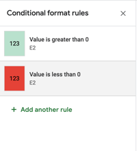
7. Return to cell to scrutinize formatting, then spin the cursor to arrange to different cells, if wanted.
Now that you just know the basics, let’s quilt simple the machine to make disclose of conditional formatting based totally solely completely on different cells.
Conditional Formatting In response to Some other Cell Designate
1. Seize the cell that you just may properly very successfully be searching to format.
2. Click on on on “Construction” inside the navigation bar, then take “Conditional Formatting.”
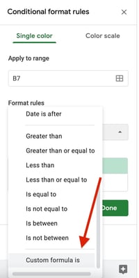
3. Underneath “Construction Tips,” take “Customized system is.”
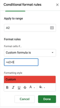
4. Write your system, then click on on “Accomplished.”
5. Verify your rule has been utilized and check out the cell.
Conditional Formatting In response to Some other Cell Fluctuate
To format based totally solely completely on one different cell differ, you put together most of the an identical steps you’d for a cell price. What changes is the system you write.
1. Seize the cell that you just may properly very successfully be searching to format.
2. Click on on on “Construction” inside the navigation bar, then take “Conditional Formatting.”
3. Underneath “Construction Tips,” take “Customized system is.”
4. Write your system the utilization of the subsequent format: =price differ < [value], take your formatting mannequin, then click on on “Accomplished.”
5. Verify your rule has been utilized and check out the cell.
Conditional Formatting In response to Some other Cell Not Empty
- Seize the cell that you just may properly very successfully be searching to format.
- Click on on on ‘Construction’ inside the navigation bar, then take ‘Conditional Formatting.’
- Underneath ‘Construction Tips,’ take ‘Customized system is.’
- Write your system the utilization of the subsequent format: =NOT(ISBLANK([cell#)), select your formatting style, then click ‘Done.’
- Confirm your rule has been applied and check the cell.
Google Sheets Conditional Formatting Based on Another Cell Color
Currently, Google Sheets does not offer a way to use conditional formatting based on the color of another cell. You can only use it based on:
- Values – higher than, greater than, equal to, in between
- Text – contains, starts with, ends with, matches
- Dates – is before, is after, is exactly
- Emptiness – is empty, is not empty
To achieve your goal, you’d have to use the condition of the cell to format the other.
Let’s use an example.
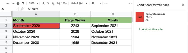
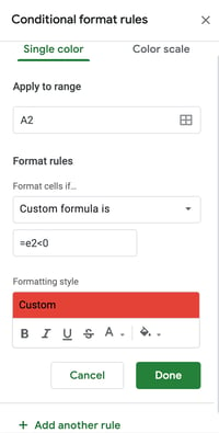
Say you want to format cell A2 (September 2020) to be red and match the color of cell E2 (-20%). There’s no formula that allows you to create a condition based on color. However, you can create a custom formula based on E2’s values.
You can say that if cell E2’s values are less than 0, cell A2 turns red. The formula is as follows: = [The other cell] < [value]. On this case, the system can be =e2<0, as a result of it implies that cell A2 may maybe silent flip pink if E2’s price is simply lower than 0.
With so many capabilities to play with, Google Sheets can appear daunting. By following these simple steps, that you just may perchance maybe simply format your cells for mercurial scanning.

Earlier than each factor printed Mar 10, 2022 7: 00: 00 AM, up to date March 10 2022