
For a great deal of entrepreneurs, trying to rearrange and analyze spreadsheets in Microsoft Excel can really feel savor strolling right into a brick wall again and again in case you’e queer with Excel formulation. You’re manually replicating columns and scribbling down long-fabricate math on a scrap of paper, all whereas considering to your self, “There has to be a bigger plan to assemble this.”
Reality be fast, there may very well be — you final get pleasure from no perception it however.
Excel may properly moreover even be difficult that plan. On the one hand, or not it is an exceptionally noteworthy device for reporting and inspecting advertising recordsdata. It’s going to even allow you visualize recordsdata with charts and pivot tables. On the alternative, with out the attractive teaching, or not it is easy to really feel savor or not it is working in opposition to you. For starters, there are further than a dozen useful formulation Excel can routinely jog for you so that you at the moment are not combing by tons of of cells with a calculator to your desk.![Accumulate 10 Excel Templates for Marketers [Free Kit]](https://no-cache.hubspot.com/cta/default/53/9ff7a4fe-5293-496c-acca-566bc6e73f42.png)
What are excel formulation?
Excel formulation allow you title relationships between values within the cells of your spreadsheet, develop mathematical calculations the utilization of those values, and return the ensuing value within the cell of your need. System it is doable you will properly maybe routinely develop encompass sum, subtraction, proportion, division, life like, and even dates/cases.
We are going to rush over all of those, and a great deal of further, on this weblog put up.
Easy ideas to Insert System in Excel
It’s doable you will properly maybe marvel what the “System” tab on the end navigation toolbar in Excel system. In further most fashionable variations of Excel, this horizontal menu — proven beneath — permits you to bag and insert Excel formulation into specific cells of your spreadsheet.
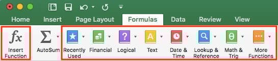
The additional you use diversified formulation in Excel, the easier it is going to seemingly be to amass into consideration them and develop them manually. On the alternative hand, the suite of icons above is a at hand catalog of formulation it is doable you will properly maybe browse and refer abet to as you hone your spreadsheet skills.
Excel formulation are each so recurrently recognized as “ideas.” To insert one into your spreadsheet, spotlight a cell by which you wish to jog a components, then click on the far-left icon, “Insert Characteristic,” to browse widespread formulation and what they assemble. That searching window will uncover savor this:
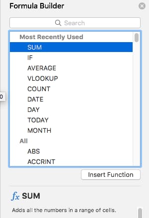 Need a further sorted searching journey? Train any of the icons now we get pleasure from highlighted (in the course of the lengthy crimson rectangle within the important screenshot above) to bag formulation linked to a differ of basic issues — equal to finance, common sense, and further. After getting stumbled on the components that fits your needs, click on “Insert Characteristic,” as proven within the window above.
Now, let’s assemble a deeper dive into a few of primarily essentially the most useful Excel formulation and tips about easy methods to develop each in conventional situations.
To allow you use Excel further successfully (and set a ton of time), now we get pleasure from compiled an inventory of useful formulation, keyboard shortcuts, and different diminutive ideas and ideas it is best to know.
NOTE: The next formulation bear in mind to essentially the most up to date mannequin of Excel. Need to you are the utilization of a a diminutive bit older mannequin of Excel, the position of every and every operate talked about beneath may properly be a diminutive bit assorted.
1. SUM
All Excel formulation start up with the equals set, =, adopted by a selected textual content set denoting the components you’d savor Excel to develop.
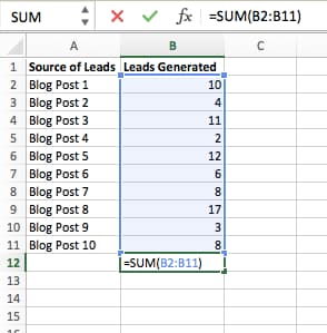
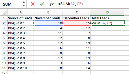
The SUM components in Excel is one amongst primarily essentially the most basic formulation it is doable you will properly maybe enter right into a spreadsheet, permitting you to bag the sum (or full) of two or further values. To develop the SUM components, enter the values you’d seize so as to add collectively the utilization of the construction, =SUM(value 1, value 2, and so forth).
The values you enter into the SUM components can both be regular numbers or equal to the quantity in a selected cell of your spreadsheet.
- To bag the SUM of 30 and 80, as an instance, kind the next components right into a cell of your spreadsheet: =SUM(30, 80). Press “Enter,” and the cell will assemble the overall of every and every numbers: 110.
- To bag the SUM of the values in cells B2 and B11, as an instance, kind the next components right into a cell of your spreadsheet: =SUM(B2, B11). Press “Enter,” and the cell will assemble the overall of the numbers on the 2nd stuffed in cells B2 and B11. If there are not any numbers in both cell, the components will return 0.
Ponder into consideration you’d moreover additionally bag the overall value of a record of numbers in Excel. To bag the SUM of the values in cells B2 by B11, kind the next components right into a cell of your spreadsheet: =SUM(B2:B11). Stage to the colon between every and every cells, reasonably than a comma. See how this is ready to properly uncover in an Excel spreadsheet for a command marketer, beneath:
2. IF
The IF components in Excel is denoted =IF(logical_test, value_if_true, value_if_false). This lets you enter a textual content value into the cell “if” one thing else on your spreadsheet is staunch or false. For instance, =IF(D2=”Gryffindor”,”10″,”0″) would award 10 ideas to cell D2 if that cell contained the phrase “Gryffindor.”
There are cases after we need to know the plan many cases a value seems to be like in our spreadsheets. However there are additionally these cases after we need to bag the cells that preserve these values, and enter specific recordsdata subsequent to it.
We are going to return to Sprung’s instance for this one. If we need to award 10 ideas to all people who belongs within the Gryffindor dwelling, reasonably than manually typing in 10’s subsequent to each Gryffindor pupil’s title, we’re going to exhaust the IF-THEN components to direct: If the pupil is in Gryffindor, then he or she should get ten ideas.
- The components: IF(logical_test, value_if_true, value_if_false)
- Logical_Test: The logical check out is the “IF” half of the assertion. On this case, the great judgment is D2=”Gryffindor.” Make sure your Logical_Test value is in citation marks.
- Value_if_True: If the fee is staunch — that is, if the pupil lives in Gryffindor — this value is the one who we need to be displayed. On this case, we need it to be the quantity 10, to notice that the pupil was awarded the ten ideas. Stage to: Easiest exhaust citation marks in case you’d savor the end result to be textual content reasonably than a quantity.
- Value_if_False: If the fee is fake — and the pupil does not reside in Gryffindor — we need the cell to display “0,” for 0 ideas.
- System in beneath instance: =IF(D2=”Gryffindor”,”10″,”0″)
3. Share
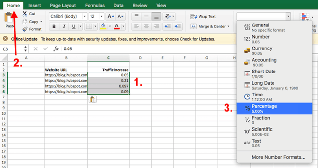
To develop the proportion components in Excel, enter the cells you’re discovering a proportion for within the construction, =A1/B1. To transform the ensuing decimal value to a proportion, spotlight the cell, click on the Dwelling tab, and preserve “Share” from the numbers dropdown.
There may very well be by no means really an Excel “components” for percentages per se, nonetheless Excel makes it simple to remodel the value of any cell right into a proportion so that you at the moment are not caught calculating and reentering the numbers your self.
The key environment to remodel a cell’s value right into a proportion is beneath Excel’s Dwelling tab. Have out this tab, spotlight the cell(s) you’d seize to remodel to a proportion, and click on on into the dropdown menu subsequent to Conditional Formatting (this menu button may properly voice “General” earlier than each little factor). Then, preserve “Share” from the record of alternate ideas that seems to be like. This is ready to properly maybe moreover convert the value of every and every cell you get pleasure from highlighted right into a proportion. See this operate beneath.
Ponder into consideration in case you’re the utilization of various formulation, such as a result of the division components (denoted =A1/B1), to return new values, your values may properly display up as decimals by default. Merely spotlight your cells before or after you develop this components, and set these cells’ construction to “Share” from the Dwelling tab — as proven above.
4. Subtraction
To develop the subtraction components in Excel, enter the cells you’re subtracting within the construction, =SUM(A1, -B1). This is ready to properly maybe moreover subtract a cell the utilization of the SUM components by including a destructive set before the cell you’re subtracting. For instance, if A1 was 10 and B1 was 6, =SUM(A1, -B1) would develop 10 + -6, returning a value of 4.
Cherish percentages, subtracting wouldn’t get pleasure from its preserve components in Excel both, nonetheless that will not indicate it may perchance perchance really’t be carried out. That you just simply can subtract any values (or these values inside cells) two assorted ideas.
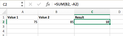
- The utilization of the =SUM components. To subtract further than one values from each different, enter the cells you’d seize to subtract within the construction =SUM(A1, -B1), with a destructive set (denoted with a hyphen) before the cell whose value you’re subtracting. Press enter to return the variation between every and every cells built-in within the parentheses. See how this seems to be like within the screenshot above.
- The utilization of the construction, =A1-B1. To subtract further than one values from each different, merely kind an equals set adopted by your first value or cell, a hyphen, and the fee or cell you’re subtracting. Press Enter to return the variation between every and every values.
5. Multiplication
To develop the multiplication components in Excel, enter the cells you’re multiplying within the construction, =A1*B1. This components makes use of an asterisk to multiply cell A1 by cell B1. For instance, if A1 was 10 and B1 was 6, =A1*B1 would return a value of 60.
It’s doable you will properly maybe state multiplying values in Excel has its preserve components or makes use of the “x” character to indicate multiplication between further than one values. Certainly, or not it is as simple as an asterisk — *.
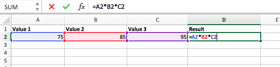
To multiply two or further values in an Excel spreadsheet, spotlight an empty cell. Then, enter the values or cells you wish to multiply collectively within the construction, =A1*B1*C1 … and so forth. The asterisk will successfully multiply each value built-in within the components.
Press Enter to return your required product. See how this seems to be like within the screenshot above.
6. Division
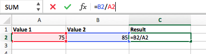
To develop the division components in Excel, enter the cells you’re dividing within the construction, =A1/B1. This components makes use of a forward scale back, “https://weblog.hubspot.com/,” to divide cell A1 by cell B1. For instance, if A1 was 5 and B1 was 10, =A1/B1 would return a decimal value of 0.5.
Division in Excel is one among the many best ideas it is doable you will properly maybe develop. To assemble so, spotlight an empty cell, enter an equals set, “=,” and bear in mind it up with the 2 (or further) values you’d seize to divide with a forward scale back, “https://weblog.hubspot.com/,” in between. The end result needs to be within the following construction: =B2/A2, as proven within the screenshot beneath.
Hit Enter, and your required quotient should appear within the cell you within the initiating highlighted.
7. DATE
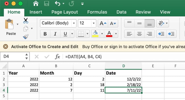
The Excel DATE components is denoted =DATE(one 12 months, month, day). This components will return a date that corresponds to the values entered within the parentheses — even values referred from different cells. For instance, if A1 was 2018, B1 was 7, and C1 was 11, =DATE(A1,B1,C1) would return 7/11/2018.
Rising dates within the cells of an Excel spreadsheet is ceaselessly a fickle project each so recurrently. Happily, there may very well be a at hand components to develop formatting your dates simple. There are two ideas to make exhaust of this components:
- Fabricate dates from a series of cell values. To assemble this, spotlight an empty cell, enter “=DATE,” and in parentheses, enter the cells whose values win your required date — beginning with the one 12 months, then the month quantity, then the day. The ultimate construction should uncover savor this: =DATE(one 12 months, month, day). See how this seems to be like within the screenshot beneath.
- Mechanically set on the unique time’s date. To assemble this, spotlight an empty cell and enter the next string of textual content: =DATE(YEAR(TODAY()), MONTH(TODAY()), DAY(TODAY())). Urgent enter will return the up to date date you’re working on your Excel spreadsheet.
In both utilization of Excel’s date components, your returned date needs to be within the fabricate of “mm/dd/yy” — except your Excel program is formatted in a totally totally different plan.
8. Array
An array components in Excel surrounds a simple components in brace characters the utilization of the construction, {=(Initiating Price 1:Finish Price 1)*(Initiating Price 2:Finish Price 2)}. By pressing ctrl+shift+heart, this is ready to properly calculate and return value from further than one ranges, reasonably than final specific specific individual cells added to or multiplied by each different.
Calculating the sum, product, or quotient of specific specific individual cells is simple — final exhaust the =SUM components and enter the cells, values, or differ of cells you wish to develop that arithmetic on. However what about further than one ranges? How assemble you gaze the combined value of a orderly neighborhood of cells?
Numerical arrays are a useful plan to develop further than one components on the equivalent time in a single cell so it is doable you will properly maybe undercover agent one remaining sum, distinction, product, or quotient. Need to you’re looking out to bag full product sales income from a number of offered items, as an instance, the array components in Excel is edifying for you. Right here is the way you’d assemble it:
- To start up the utilization of the array components, kind “=SUM,” and in parentheses, enter the first of two (or three, or 4) ranges of cells you’d seize to multiply collectively. This is what your improvement may properly uncover savor: =SUM(C2:C5
- Subsequent, add an asterisk after the final cell of the numerous differ you built-in on your components. This stands for multiplication. Following this asterisk, enter your 2nd differ of cells. It’s doable you will properly be multiplying this 2nd differ of cells by the numerous. Your improvement on this components should now uncover savor this: =SUM(C2:C5*D2:D5)
- Prepared to press Enter? Not so fleet … As a result of this components is so advanced, Excel reserves a assorted keyboard stammer for arrays. After getting closed the parentheses to your array components, press Ctrl+Shift+Enter. This is ready to properly maybe moreover survey your components as an array, wrapping your components in brace characters and effectively returning your manufactured from every and every ranges combined.
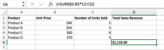
In income calculations, this is ready to properly cleave abet right down to your time and power severely. See the ultimate components within the screenshot above.
9. COUNT
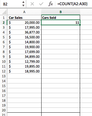
The COUNT components in Excel is denoted =COUNT(Initiating Cell:Finish Cell). This components will return a value that’s the equivalent as a result of the quantity of entries stumbled on inside your required differ of cells. For instance, if there are eight cells with entered values between A1 and A10, =COUNT(A1:A10) will return a value of 8.
The COUNT components in Excel is extremely useful for orderly spreadsheets, whereby you wish to survey what variety of cells preserve regular entries. Don’t be fooled: This components won’t assemble any math on the values of the cells themselves. This components is barely to bag out what variety of cells in a selected differ are targeted on one thing.
The utilization of the components in courageous above, it is doable you will properly maybe effortlessly jog a rely of transferring cells on your spreadsheet. The end result will uncover a diminutive one thing savor this:
10. AVERAGE
To develop the smartly-liked components in Excel, enter the values, cells, or differ of cells of which you’re calculating the smartly-liked within the construction, =AVERAGE(number1, number2, and so forth.) or =AVERAGE(Initiating Price:Finish Price). This is ready to properly maybe moreover calculate the smartly-liked of the total values or differ of cells built-in within the parentheses.
Discovering the smartly-liked of a differ of cells in Excel retains you from having to bag specific specific individual sums after which performing a separate division equation to your full. The utilization of =AVERAGE as your preliminary textual content entry, it is doable you will properly maybe let Excel assemble the total provide the outcomes you need.
For reference, the smartly-liked of a neighborhood of numbers is the equivalent as a result of the sum of those numbers, divided by the quantity of issues in that neighborhood.
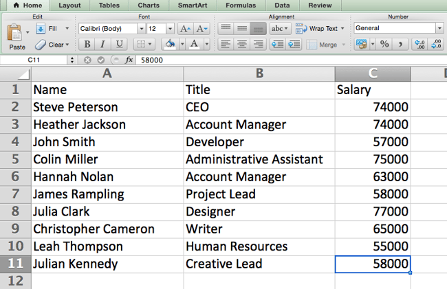
11. SUMIF
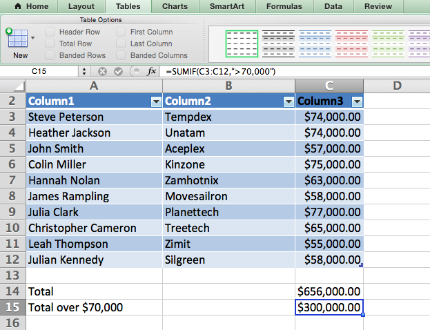
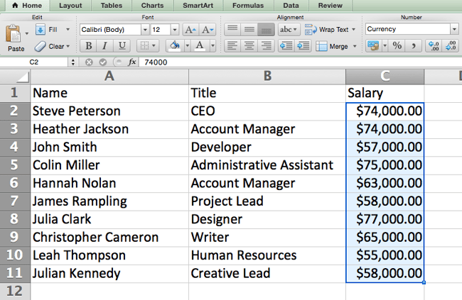
The SUMIF components in Excel is denoted =SUMIF(differ, standards, [sum range]). This is ready to properly maybe moreover return the sum of the values inside a desired differ of cells that each one meet one criterion. For instance, =SUMIF(C3:C12,”>70,000″) would return the sum of values between cells C3 and C12 from easiest the cells which can be bigger than 70,000.
For example you wish to bag out the revenue you generated from an inventory of leads who’re linked to specific dwelling codes, or calculate the sum of sure employees’ salaries — nonetheless easiest in the event that they drop above a selected quantity. Doing that manually sounds a diminutive time-drinking, to direct the least.
With the SUMIF operate, it could not want to be — it is doable you will properly maybe effortlessly add up the sum of cells that meet sure standards, savor within the wage instance above.
- The components: =SUMIF(differ, standards, [sum_range])
- Differ: The differ that is being examined the utilization of your standards.
- Standards: The elements that resolve which cells in Criteria_range1 will seemingly be added collectively
- [Sum_range]: An elective differ of cells you’ll add up as properly to to the numerous Differ entered. This self-discipline may properly moreover very well be uncared for.
Within the occasion beneath, we wished to calculate the sum of the salaries that had been bigger than $70,000. The SUMIF operate added up the buck quantities that exceeded that amount within the cells C3 by C12, with the components =SUMIF(C3:C12,”>70,000″).
12. TRIM
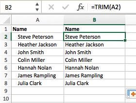
The TRIM components in Excel is denoted =TRIM(textual content). This components will seize any areas entered before and after the textual content entered within the cell. For instance, if A2 entails the title ” Steve Peterson” with undesirable areas before the numerous title, =TRIM(A2) would return “Steve Peterson” and not using a areas in a brand new cell.
Piece of email and file sharing are acceptable devices in on the unique time’s map of labor. That’s, until one amongst your colleagues sends you a worksheet with some really funky spacing. Not easiest can these rogue areas develop it advanced to survey for recordsdata, nonetheless as properly they get pleasure from an set on the outcomes everytime you occur to try so as to add up columns of numbers.
In need to painstakingly pushing apart and including areas as needed, it is doable you will properly maybe orderly up any irregular spacing the utilization of the TRIM operate, which is passe to seize further areas from recordsdata (apart from single areas between phrases).
- The components: =TRIM(textual content).
- Textual content: The textual content or cell from which you wish to seize areas.
Right here is an instance of how we passe the TRIM operate to seize further areas before an inventory of names. To assemble so, we entered =TRIM(“A2”) into the System Bar, and replicated this for each title beneath it in a brand new column subsequent to the column with undesirable areas.
Under are another Excel formulation it is doable you will properly maybe bag useful as your recordsdata administration needs develop.
13. LEFT, MID, and RIGHT
For example you get pleasure from a line of textual content inside a cell that you simply really need to present plan into a few assorted segments. In need to manually retyping each share of the code into its respective column, clients can leverage a series of string ideas to deconstruct the sequence as needed: LEFT, MID, or RIGHT.
LEFT
- Draw: Weak to extract the numerous X numbers or characters in a cell.
- The components: =LEFT(textual content, number_of_characters)
- Textual content: The string that you simply seize to extract from.
- Number_of_characters: The quantity of characters that you simply seize to extract ranging from the left-most character.
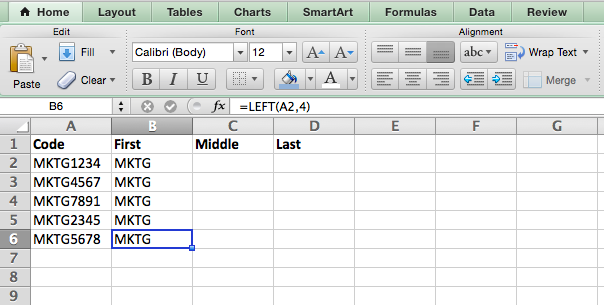
Within the occasion beneath, we entered =LEFT(A2,4) into cell B2, and copied it into B3:B6. That allowed us to extract the numerous 4 characters of the code.
MID
- Draw: Weak to extract characters or numbers within the heart consistent with map.
- The components: =MID(textual content, start_position, number_of_characters)
- Textual content: The string that you simply seize to extract from.
- Start_position: The map within the string that you simply really need to start up extracting from. For instance, the numerous map within the string is 1.
- Number_of_characters: The quantity of characters that you simply seize to extract.
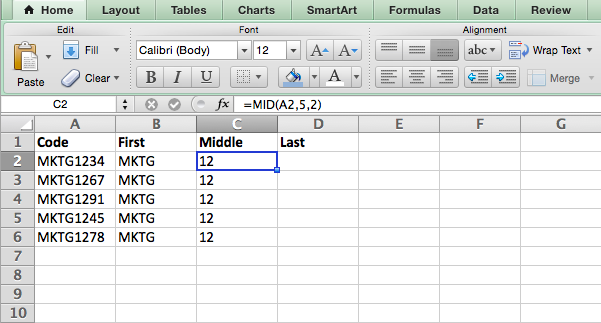
On this case, we entered =MID(A2,5,2) into cell B2, and copied it into B3:B6. That allowed us to extract the 2 numbers beginning within the fifth map of the code.
RIGHT
- Draw: Weak to extract the final X numbers or characters in a cell.
- The components: =RIGHT(textual content, number_of_characters)
- Textual content: The string that you simply seize to extract from.
- Number_of_characters: The quantity of characters that you simply really need to extract ranging from the gorgeous-most character.
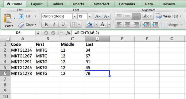
For the sake of this case, we entered =RIGHT(A2,2) into cell B2, and copied it into B3:B6. That allowed us to extract the final two numbers of the code.
14. VLOOKUP
This one is an oldie, nonetheless a goodie — and or not it is miles a diminutive further broad than one of the most different formulation now we get pleasure from listed right here. However or not it is particularly priceless for these cases everytime you occur to get pleasure from two items of knowledge on two assorted spreadsheets, and need to mix them right into a single spreadsheet.
My colleague, Rachel Sprung — whose “Easy ideas to Train Excel” tutorial is a have to-read for anyone who needs to study — makes use of an inventory of names, e mail addresses, and corporations as an instance. Need to you get pleasure from an inventory of of us’s names subsequent to their e mail addresses in a single spreadsheet, and an inventory of those equivalent of us’s e mail addresses subsequent to their firm names within the reverse, nonetheless you need the names, e mail addresses, and firm names of those of us to look in a single map — that’s the win VLOOKUP is accessible in.
Stage to: When the utilization of this components, it is best to make sure that no lower than one column seems to be like identically in every and every spreadsheets. Scour your recordsdata items to make sure that the column of knowledge you are the utilization of to mix your recordsdata is strictly the equivalent, collectively and not using a further areas.
- The components: VLOOKUP(lookup value, desk array, column quantity, [range lookup])
- Lookup Price: The equivalent value you get pleasure from in every and every spreadsheets. Blueprint discontinuance the numerous value on your first spreadsheet. In Sprung’s instance that follows, this implies the numerous e mail deal with on the record, or cell 2 (C2).
- Desk Array: The differ of columns on Sheet 2 you’ll drag your recordsdata from, together with the column of knowledge equivalent to your lookup value (in our instance, e mail addresses) in Sheet 1 as properly to the column of knowledge you are attempting to duplicate to Sheet 1. In our instance, that’s “Sheet2!A:B.” “A” system Column A in Sheet 2, which is the column in Sheet 2 the win the information equivalent to our lookup value (e mail) in Sheet 1 is listed. The “B” system Column B, which includes the information that is easiest accessible in Sheet 2 that you simply really need to translate to Sheet 1.
- Column Quantity: The desk array tells Excel the win (which column) the model new recordsdata you wish to duplicate to Sheet 1 is positioned. In our instance, this is ready to properly be the “Rental” column, the 2nd one in our desk array, making it column quantity 2.
- Differ Lookup: Train FALSE to make sure you pull in easiest regular value fits.
- The components with variables from Sprung’s instance beneath: =VLOOKUP(C2,Sheet2!A:B,2,FALSE)
On this case, Sheet 1 and Sheet 2 preserve lists describing assorted details in regards to the equivalent of us, and the basic thread between the 2 is their e mail addresses. For example we need to mix every and every datasets in declare that the total dwelling recordsdata from Sheet 2 interprets over to Sheet 1. Right here is how that may properly work:
15. RANDOMIZE
There may very well be an enormous article that likens Excel’s RANDOMIZE components to shuffling a deck of taking part in playing cards. The whole deck is a column, and every card — 52 in a deck — is a row. “To gallop the deck,” writes Steve McDonnell, “it is doable you will properly maybe compute a brand new column of knowledge, populate each cell within the column with a random quantity, and kind the workbook consistent with the random quantity self-discipline.”
In advertising, it is doable you will properly maybe exhaust this operate everytime you occur to need to win a random quantity to an inventory of contacts — savor in case you wished to experiment with a brand new e mail marketing campaign and needed to make exhaust of blind standards to win who would win it. By assigning numbers to acknowledged contacts, you’d moreover bear in mind the rule of thumb, “Any contact with a resolve of 6 or above will seemingly be added to the model new marketing campaign.”
- The components: RAND()
- Initiating with a single column of contacts. Then, within the column adjoining to it, kind “RAND()” — with out the citation marks — beginning with the end contact’s row.
- RANDBETWEEN permits you to dictate the differ of numbers that you simply really need to be assigned. Within the case of this case, I wanted to make exhaust of 1 by 10.
- backside: The bottom quantity within the differ.
- high: The supreme quantity within the differ,For the occasion beneath: RANDBETWEEN(backside,high)
- System in beneath instance: =RANDBETWEEN(1,10)
Important stuff, attractive? Now for the icing on the cake: After getting mastered the Excel components you need, you’ll want to replicate it for different cells with out rewriting the components. And by chance, there may very well be an Excel operate for that, too. Try it out beneath.
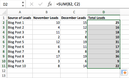
As soon as in a while, it is doable you will properly maybe want to jog the equivalent components throughout an entire row or column of your spreadsheet. For example, as an instance, you get pleasure from an inventory of numbers in columns A and B of a spreadsheet and need to enter specific specific individual totals of every and every row into column C.
Clearly, it would be too unhurried to change the values of the components for each cell so you’re discovering the overall of every and every row’s respective numbers. Happily, Excel permits you to routinely full the column; all or not it is miles wanted to assemble is enter the components within the important row. Check out the next steps:
- Kind your components into an empty cell and press “Enter” to jog the components.

- Hover your cursor over the underside-gorgeous nook of the cell containing the components. It’s doable you will properly undercover agent a diminutive, courageous “+” image seem.
- Whereas it is doable you will properly maybe double-click this image to routinely soak up the ultimate column alongside together with your components, you’d moreover additionally click on and sprint your cursor down manually to soak up easiest a selected size of the column.
 After getting reached the final cell within the column you’d seize to enter your components, liberate your mouse to duplicate the components. Then, merely check out each new value to make sure it corresponds to the staunch cells.
 After getting reached the final cell within the column you’d seize to enter your components, liberate your mouse to duplicate the components. Then, merely check out each new value to make sure it corresponds to the staunch cells.
Excel Keyboard Shortcuts
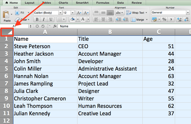
1. Quickly preserve rows, columns, or your full spreadsheet.
Most most seemingly you’re crunched for time. I indicate, who is rarely really? No time, no direct. That you just simply can preserve your full spreadsheet in only one click on. All or not it is miles wanted to assemble is barely click on the tab within the finish-left nook of your sheet to concentrate on each little factor .
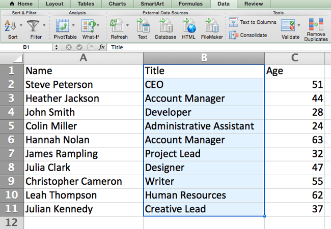
Honest correct want to win each little factor in a selected column or row? That’s final as simple with these shortcuts:
For Mac:
- Have out Column = Direct + Shift + Down/Up
- Have out Row = Direct + Shift + Honest correct/Left
For PC:
- Have out Column = Comprise watch over + Shift + Down/Up
- Have out Row = Comprise watch over + Shift + Honest correct/Left
This shortcut is mainly priceless everytime you occur to are working with bigger recordsdata items, nonetheless easiest want to win a selected share of it.
2. Quickly open, discontinuance, or win a workbook.
Comprise to open, discontinuance, or win a workbook on the wing? The next keyboard shortcuts will relieve you full any of the above actions in lower than a minute’s time.
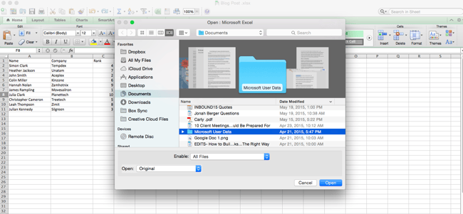
For Mac:
- Initiating = Direct + O
- Conclude = Direct + W
- Fabricate Modern = Direct + N
For PC:
- Initiating = Comprise watch over + O
- Conclude = Comprise watch over + F4
- Fabricate Modern = Comprise watch over + N
3. Format numbers into forex.
Comprise raw recordsdata that you simply really need to flip into forex? Whether or not it’s wage figures, advertising budgets, or ticket product sales for an match, the reply is simple. Honest correct spotlight the cells you seize to reformat, and preserve Comprise watch over + Shift + $.
The numbers will routinely translate into buck quantities — full with buck indicators, commas, and decimal ideas.
Stage to: This shortcut additionally works with percentages. Need to you wish to imprint a column of numerical values as “%” figures, substitute “$” with “%”.
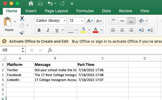
4. Insert up to date date and time right into a cell.
Whether or not you’re logging social media posts, or conserving music of duties you’re checking off your to-construct record, it is doable you will properly maybe want to add a date and time value to your worksheet. Initiating by choosing the cell to which you want so as to add this information.
Then, depending on what you wish to insert, assemble one among the many following:
- Insert up to date date = Comprise watch over + ; (semi-colon)
- Insert up to date time = Comprise watch over + Shift + ; (semi-colon)
- Insert up to date date and time = Comprise watch over + ; (semi-colon), SPACE, after which Comprise watch over + Shift + ; (semi-colon).
Different Excel Solutions
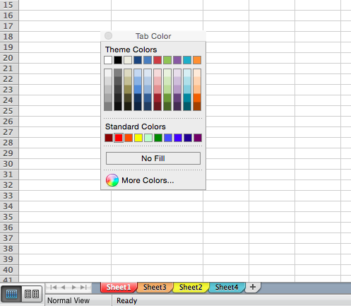
1. Customise the colour of your tabs.
Need to you get pleasure from a ton of varied sheets in a single workbook — which happens to the bigger of us — develop it easier to title the win or not it is miles wanted to move by color-coding the tabs. For instance, it is doable you will properly maybe imprint final month’s advertising experiences with crimson, and this month’s with orange.
Merely attractive click on a tab and preserve “Tab Color.” A popup will seem that lets you win a shade from an unique theme, or customise one to satisfy your needs.
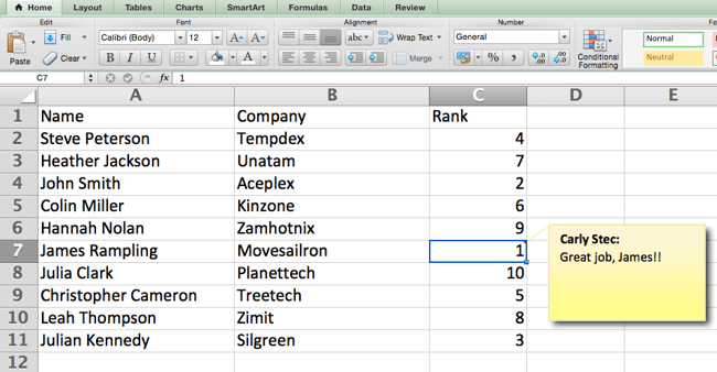
2. Add a remark to a cell.
Need to you wish to develop a word or add a remark to a selected cell inside a worksheet, merely gorgeous-click the cell you want to the touch upon, then click on Insert Remark. Kind your remark into the textual content discipline, and click on on outside the remark discipline to place it aside.
Cells that preserve feedback word a diminutive, crimson triangle within the nook. To leer the remark, skim over it.
3. Copy and replica formatting.
Need to you get pleasure from ever spent a while formatting a sheet to your liking, you presumably agree that or not it is not precisely primarily essentially the most good-looking mumble. Actually, or not it is reasonably unhurried.
For that cause, or not it is seemingly that you simply should not have to repeat the trail of subsequent time — nor assemble or not it is miles wanted to. Which capability of Excel’s Format Painter, it is doable you will properly maybe effortlessly duplicate the formatting from one dwelling of a worksheet to another.
Have out what you’d seize to duplicate, then preserve the Format Painter risk — the paintbrush icon — from the dashboard. The pointer will then word a paintbrush, prompting you to win the cell, textual content, or full worksheet to which you wish to bear in mind that formatting, as proven beneath:
.gif?width=650&name=Copy%20Duplicate%20Formatting%20(1).gif)
4. Identify replica values.
In lots of circumstances, replica values — savor replica command when managing search engine optimisation — may properly moreover even be troublesome if gone uncorrected. In some situations, even though, you simply want to be attentive to it.
Whatever the misery may properly moreover very well be, or not it is easy to floor any unique replica values inside your worksheet in near a fleet steps. To assemble so, click on into the Conditional Formatting risk, and preserve Highlight Cell Rules > Duplicate Values
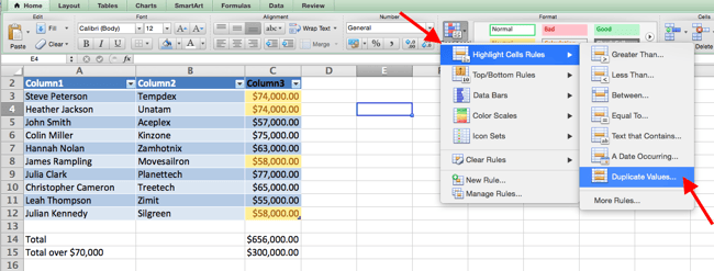
The utilization of the popup, win the specified formatting rule to specify which fabricate of replica command you seize to carry forward.
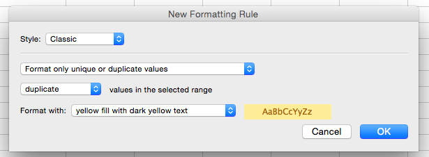
Within the occasion above, we had been searching to title any replica salaries inside the chosen differ, and formatted the replica cells in yellow.
Excel Shortcuts Place You Time
In advertising, the exhaust of Excel is reasonably inevitable — nonetheless with these ideas, it could not want to be so daunting. As they voice, bear in mind makes edifying. The additional you use these formulation, shortcuts, and ideas, the additional they might properly develop into 2nd nature.
Editor’s word: This put up was within the initiating printed in January 2019 and has been up to this point for comprehensiveness.


Initially printed Jul 27, 2022 7: 00: 00 AM, up to this point July 27 2022