![the-draw-to-accomplish-a-chart-or-graph-in-excel-[with-video-tutorial]](https://technewsedition.com/wp-content/uploads/2022/09/7510-the-draw-to-accomplish-a-chart-or-graph-in-excel-with-video-tutorial.jpg-23keepProtocol)
Setting up charts and graphs are one in all many handiest strategies to visualise recordsdata in a transparent and understandable method.
Nonetheless, or now not it’s no shock that some folks procure reasonably intimidated by the prospect of poking spherical in Microsoft Excel.

I assumed I would fragment a suited video tutorial other than a pair step-by-step directions for anybody out there who cringes on the perception to be organizing a spreadsheet plump of recordsdata exact right into a chart that in fact, you realize, method one factor. However ahead of diving in, we should all the time hurry over the diversified kinds of charts you may perchance perchance per likelihood per likelihood glean within the scheme.
Types of Charts in Excel
You’ll be able to execute further than lovely bar or line charts in Microsoft Excel, and when the makes use of for each, you may perchance perchance per likelihood per likelihood design further insightful recordsdata in your or your physique of employees’s initiatives.
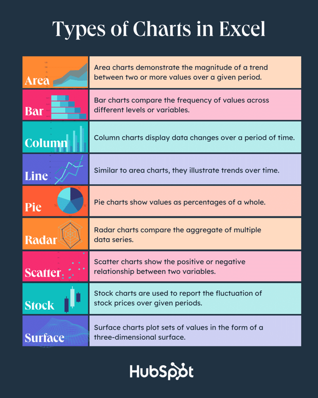
Type of Chart | Expend |
Predicament | Predicament charts exhibit the magnitude of a mannequin between two or further values over a given period. |
Bar | Bar charts evaluate the frequency of values throughout diversified ranges or variables. |
Column | Column charts exhibit recordsdata modifications or a timeframe. |
Line | Similar to bar charts, they illustrate developments over time. |
Pie | Pie charts inform values as percentages of a full. |
Radar | Radar charts evaluate the mixture of a pair of recordsdata sequence. |
Scatter | Scatter charts inform the certain or detrimental relationship between two variables. |
Stock | Stock charts are aged to yarn the fluctuation of inventory prices over given intervals. |
Floor | Floor charts area devices of values within the assemble of a 3-D ground. |
The steps or now not it’s a should enjoyment of to assemble a chart or graph in Excel are simple, and right here’s a brief walkthrough on execute them.
Take be aware there are a broad variety of diversified variations of Excel, so what you peek within the video above may perchance perchance now not all the time match up exactly with what you are going to peek in your model. Throughout the video, I aged Excel 2021 model 16.49 for Mac OS X.
To obtain probably the most up to date directions, I abet you to please in a have a look at the written directions under (or protected them as PDFs). Lots of the buttons and features you are going to peek and skim are very an equivalent throughout all variations of Excel.
Accumulate Demo Data | Accumulate Directions (Mac) | Accumulate Directions (PC)
The draw to Accomplish a Graph in Excel
- Enter your recordsdata into Excel.
- Expend one in all 9 graph and chart options to execute.
- Highlight your recordsdata and click on on ‘Insert’ your required graph.
- Swap the solutions on each axis, if wished.
- Modify your recordsdata’s format and colours.
- Commerce the dimensions of your chart’s delusion and axis labels.
- Commerce the Y-axis measurement options, if desired.
- Reorder your recordsdata, if desired.
- Title your graph.
- Export your graph or chart.
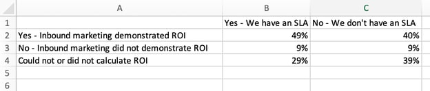
1. Enter your recordsdata into Excel.
First, or now not it’s a should enjoyment of to enter your recordsdata into Excel. You are going to please in exported the solutions from in diversified areas, relish a portion of selling scheme or a search scheme. Or possibly you may perchance perchance per likelihood be inputting it manually.
Throughout the occasion under, in Column A, I in fact enjoyment of a guidelines of responses to the inquire, “Did inbound promoting exhibit ROI?”, and in Columns B, C, and D, I in fact delight within the responses to the inquire, “Does your group enjoyment of a proper sales-advertising settlement?” For example, Column C, Row 2 illustrates that 49% of folks with a service degree settlement (SLA) furthermore advise that inbound promoting demonstrated ROI.
2. Expend from the graph and chart options.
In Excel, your options for charts and graphs embody column (or bar) graphs, line graphs, pie graphs, scatter plots, and additional. Scrutinize how Excel identifies each within the head navigation bar, as depicted under:
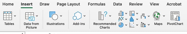
To hunt out the chart and graph options, glean out Insert.
(For assist realizing which type of chart/graph is handiest for visualizing your recordsdata, check out out our free e information, The draw to Expend Data Visualization to Procure shut Over Your Viewers.)
3. Highlight your recordsdata and insert your required graph into the spreadsheet.
On this occasion, a bar graph affords the solutions visually. To execute a bar graph, highlight the solutions and embody the titles of the X and Y-axis. Then, hurry to the Insert tab and click on on the column icon within the charts allotment. Expend the graph you should have from the dropdown window that appears.
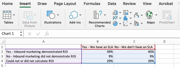
I picked the predominant two dimensional column choice on delusion of I glean the flat bar graphic over the three dimensional peek. Scrutinize the ensuing bar graph under.
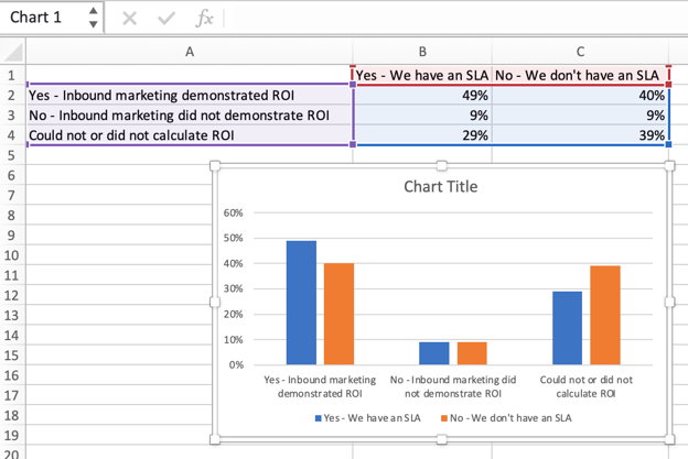
4. Swap the solutions on each axis, if wished.
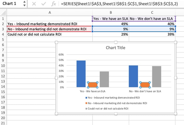
While you may perchance perchance per likelihood wish to swap what appears on the X and Y axis, lawful-click on on the bar graph, click on on Expend Data, and click on on Swap Row/Column. This may perchance perchance rearrange which axes raise which objects of recordsdata within the guidelines proven under. When completed, click on on OK on the backside.
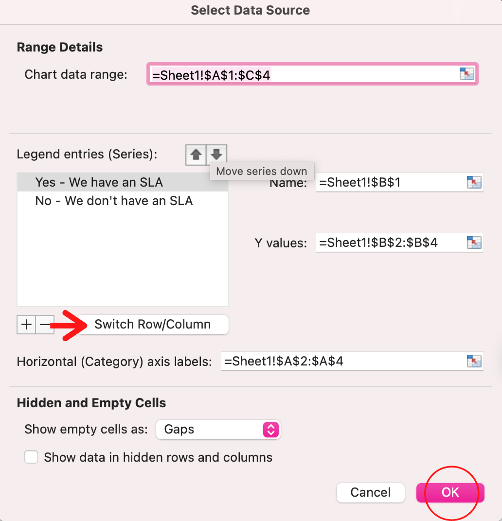
The ensuing graph would peek relish this:
5. Modify your recordsdata’s format and colours.
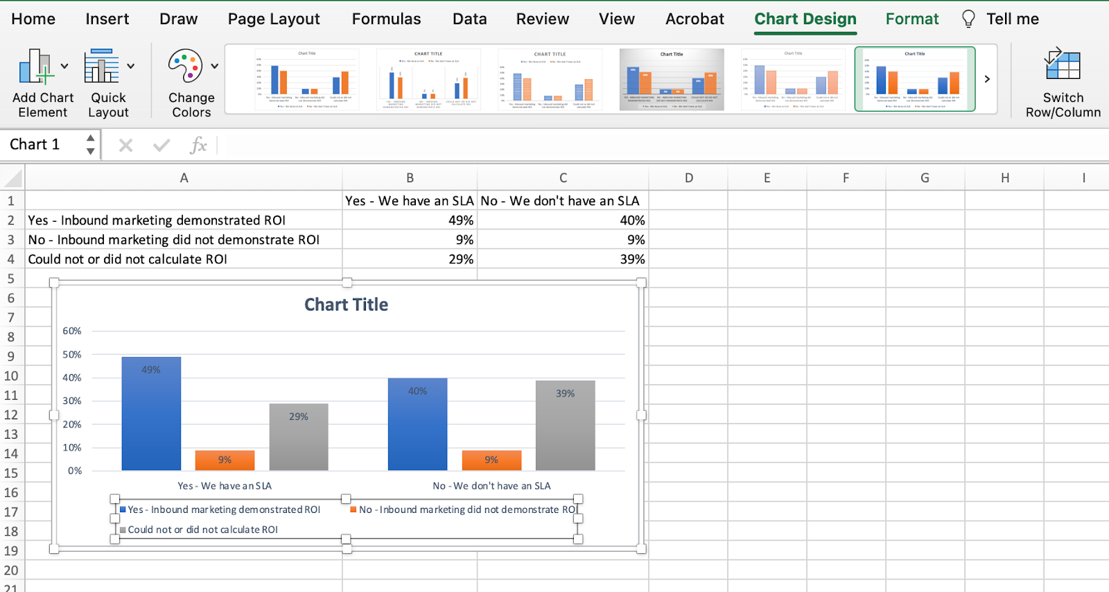
To commerce the labeling format and delusion, click on on on the bar graph, then click on on the Chart Produce tab. Proper right here, you may perchance perchance per likelihood per likelihood protected which format to obtain for the chart title, axis titles, and delusion. In my occasion under, I clicked on the prospect that displayed softer bar colours and legends under the chart.
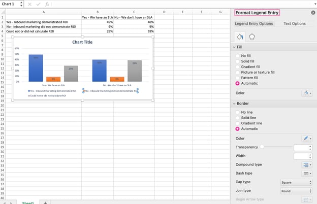
To further format the parable, click on on on it as an example the Format Epic Entry sidebar, as proven under. Proper right here, you may perchance perchance per likelihood per likelihood commerce the glean coloration of the parable, that might unprejudiced commerce the coloration of the columns themselves. To format different substances of your chart, click on on on them in my thought as an example a corresponding Format window.
6. Commerce the dimensions of your chart’s delusion and axis labels.
Throughout the occasion you first execute a graph in Excel, the dimensions of your axis and delusion labels may perchance perchance unprejudiced be little, counting on the graph or chart to obtain (bar, pie, line, and so forth.) After getting created your chart, you are going to would in fact like to provide a protected to those labels so that they’re legible.
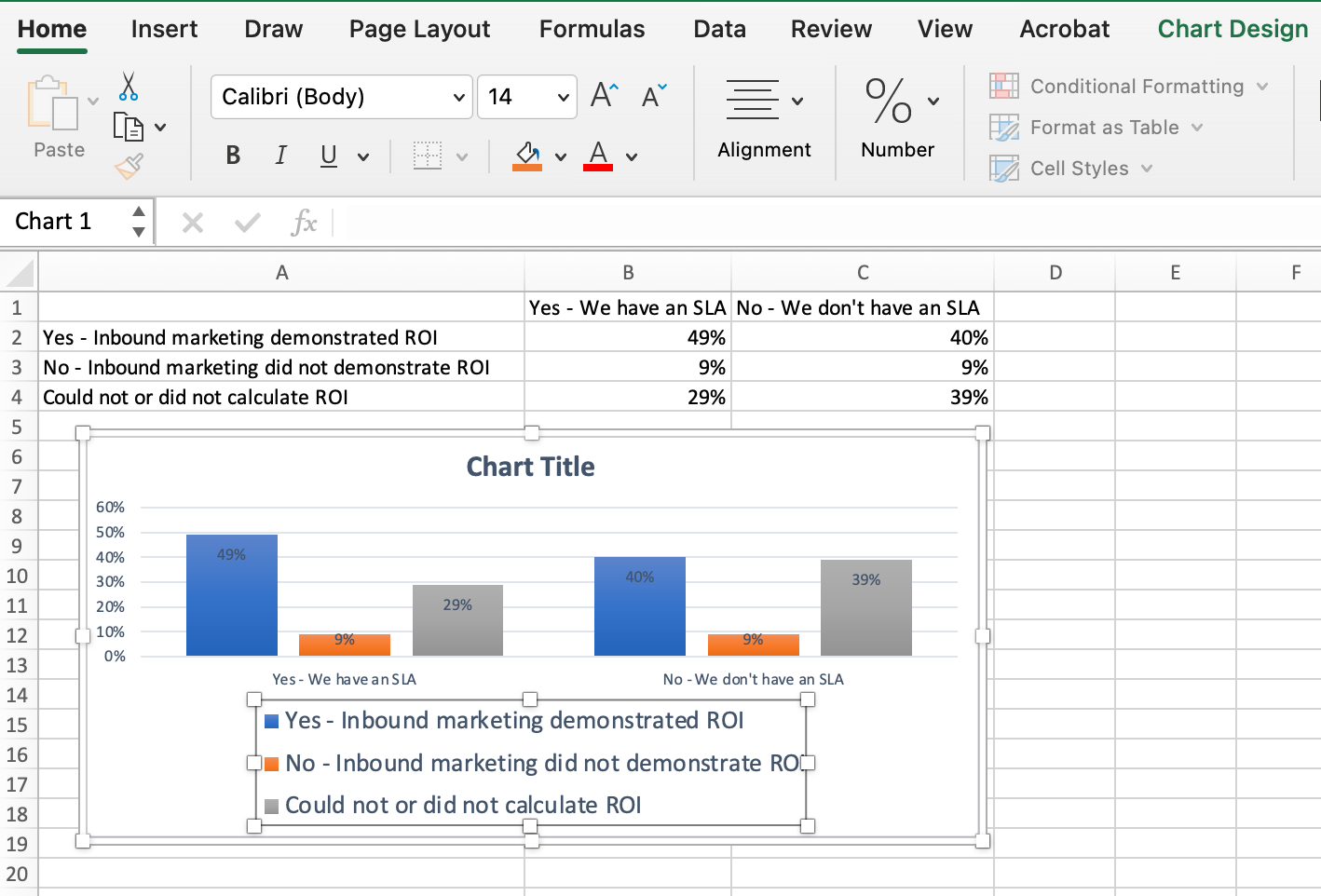
To elongate the dimensions of your graph’s labels, click on on on them in my thought and, as an alternate of unveiling a model new Format window, click on on once more into the Dwelling tab within the head navigation bar of Excel. Then, use the font kind and measurement dropdown fields to elongate or shrink your chart’s delusion and axis labels to your liking.
7. Commerce the Y-axis measurement options if desired.
To commerce the type of measurement proven on the Y axis, click on on on the Y-axis percentages in your chart as an example the Format Axis window. Proper right here, you may perchance perchance per likelihood per likelihood protected everytime you occur to’d relish as an example devices positioned on the Axis Alternate selections tab, or everytime you occur to’d relish to commerce whether or not the Y-axis reveals percentages to 2 decimal areas or no decimal areas.
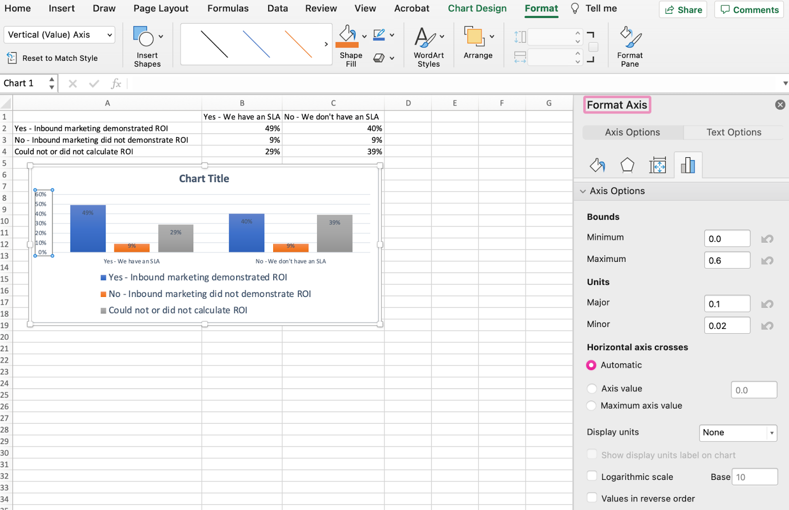
As a result of my graph mechanically devices the Y axis’s most share to 60%, you are going to doubtlessly would in fact wish to commerce it manually to 100% to indicate my recordsdata on a common scale. To develop so, you may perchance perchance per likelihood per likelihood glean out the Most choice — two fields down under Bounds within the Format Axis window — and commerce the value from 0.6 to 1.
The ensuing graph will peek relish the one under (On this occasion, the font measurement of the Y-axis has been elevated by means of the Dwelling tab so that you just may perchance perchance per likelihood per likelihood peek the variation):

8. Reorder your recordsdata, if desired.
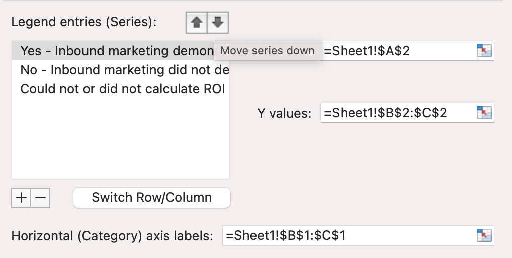
To kind the solutions so the respondents’ options appear in reverse inform, lawful-click on in your graph and click on on Expend Data as an example the identical options window you often known as up in Step 3 above. This time, arrow up and right down to reverse the inform of your recordsdata on the chart.
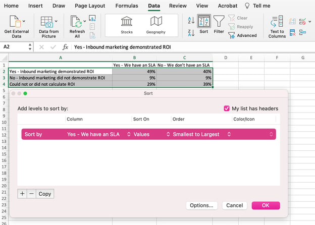
While you enjoyment of further than two traces of recordsdata to change, you may perchance perchance per likelihood per likelihood furthermore rearrange them in ascending or descending inform. To develop this, highlight your complete recordsdata within the cells above your chart, click on on Data and protected out Type, as proven under. Reckoning in your choice, you may perchance perchance per likelihood per likelihood protected to kind per smallest to ideally fantastic, or vice versa.
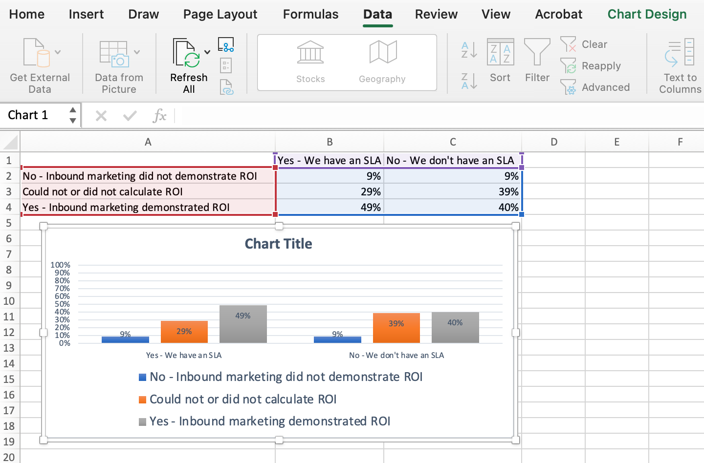
The ensuing graph would peek relish this:
9. Title your graph.
Now comes the enjoyable and easy fragment: naming your graph. By now, you may perchance perchance per likelihood enjoyment of already found develop that. Proper this is a simple clarifier.
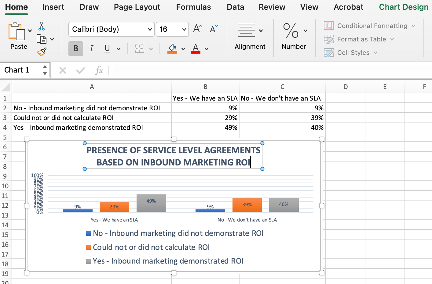
Lawful after making your chart, the title that appears will seemingly be “Chart Title,” or one factor an equivalent counting on the model of Excel you may perchance perchance per likelihood be using. To commerce this designate, click on on on “Chart Title” as an example a typing cursor. You’ll be able to then freely customise your chart’s title.
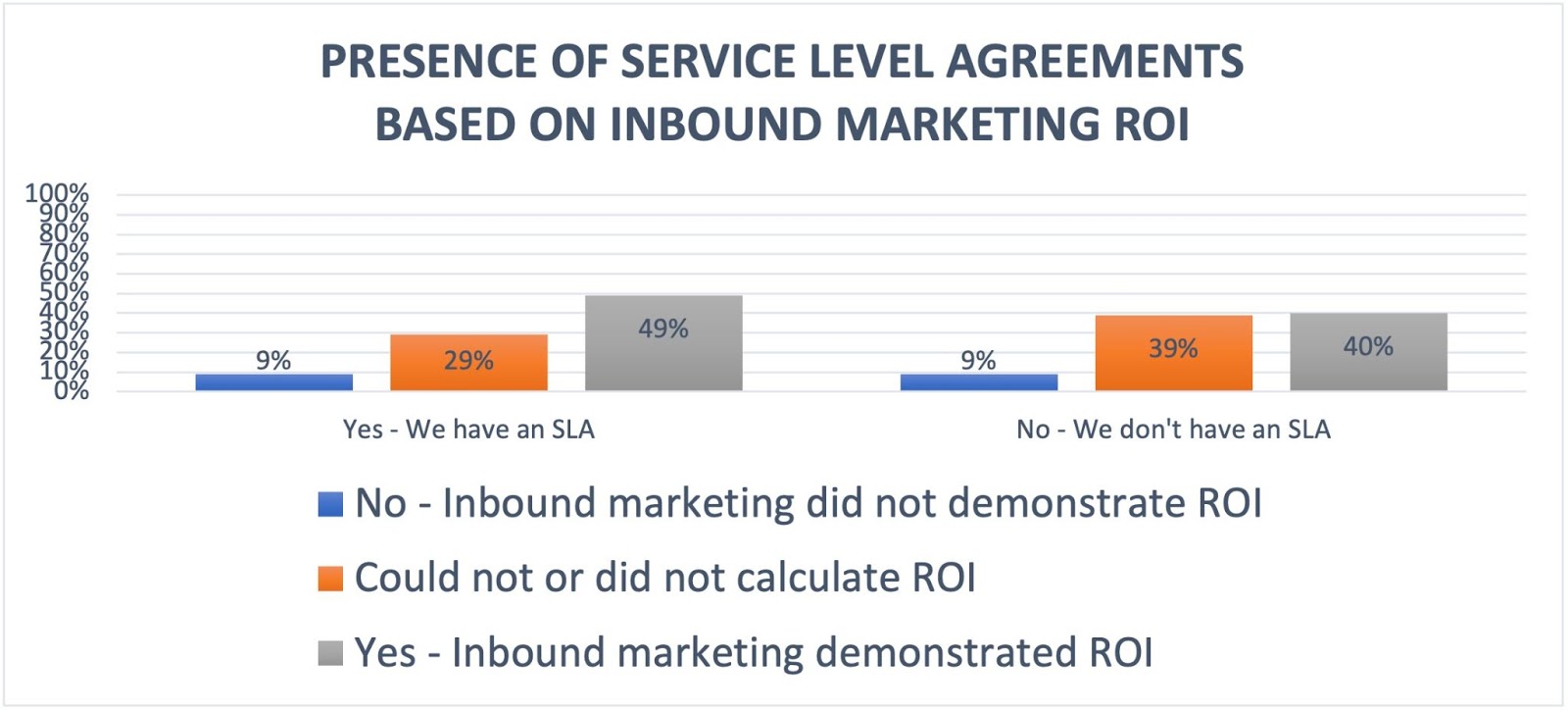
Throughout the occasion you enjoyment of a title you relish, click on on Dwelling on the pinnacle navigation bar, and use the font formatting options to provide your title the emphasis it deserves. Scrutinize these options and my closing graph under:
10. Export your graph or chart.
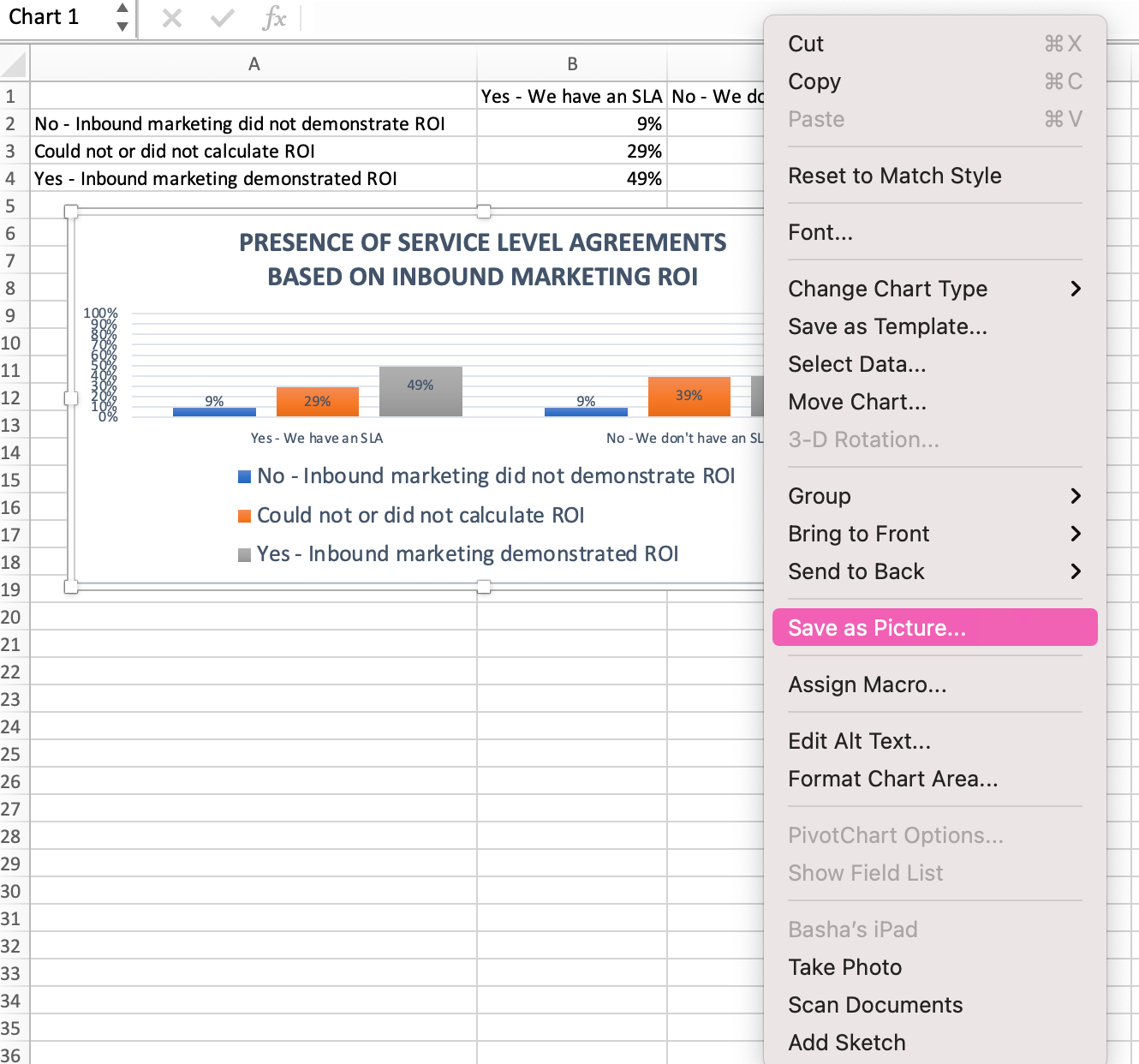
As soon as your chart or graph is exactly the draw you favor it, you may perchance perchance per likelihood per likelihood connect it as a picture with out screenshotting it within the spreadsheet. This implies provides you with a tidy picture of your chart that can also be inserted exact right into a PowerPoint presentation, Canva doc, or one other visible template.
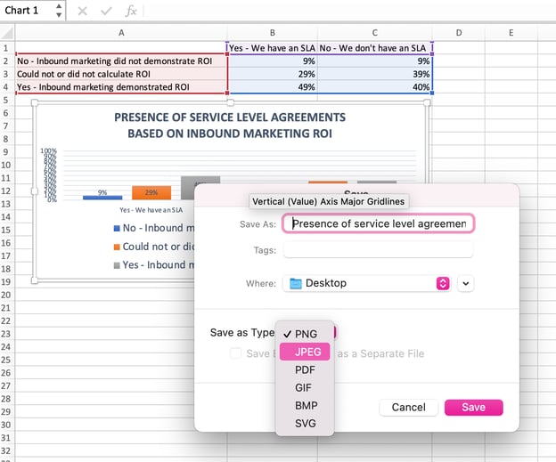
To connect your Excel graph as a photograph, lawful-click on on the graph and protected out Set as Characterize.
Throughout the dialogue field, identify the picture of your graph, protected the place to connect it in your laptop computer, and protected the file kind you’d relish to connect it as. On this occasion, it’s saved as a JPEG to a desktop folder. Lastly, click on on Set.
You’ll enjoyment of a transparent picture of your graph or chart that you just may perchance perchance per likelihood per likelihood add to any visible assemble.
Visualize Data Love A Educated
That grew to become as quickly as fairly simple, lawful? With this step-by-step tutorial, you’ll be able to fleet glean charts and graphs that visualize probably the most sophisticated recordsdata. Attempt using this similar tutorial with diversified graph kinds relish a pie chart or line graph to peek what format tells the yarn of your recordsdata handiest.
Editor’s point out: This publish grew to become as quickly as on the origin printed in June 2018 and has been up to date for comprehensiveness.

Initially printed Sep 8, 2022 7: 00: 00 AM, up to date September 08 2022